Bayesian Neural Network

We borrow this tutorial from the official Turing Docs. We will show how the explicit parameterization of Lux enables first-class composability with packages which expect flattened out parameter vectors.

Note: The tutorial in the official Turing docs is now using Lux instead of Flux.

We will use Turing.jl with Lux.jl to implement implementing a classification algorithm. Lets start by importing the relevant libraries.

# Import libraries

using Lux, Turing, CairoMakie, Random, Tracker, Functors, LinearAlgebra

# Sampling progress
Turing.setprogress!(true);

[ Info: [Turing]: progress logging is enabled globally
[ Info: [AdvancedVI]: global PROGRESS is set as true

Generating data

Our goal here is to use a Bayesian neural network to classify points in an artificial dataset. The code below generates data points arranged in a box-like pattern and displays a graph of the dataset we'll be working with.

# Number of points to generate
N = 80
M = round(Int, N / 4)
rng = Random.default_rng()
Random.seed!(rng, 1234)

# Generate artificial data
x1s = rand(rng, Float32, M) * 4.5f0;
x2s = rand(rng, Float32, M) * 4.5f0;
xt1s = Array([[x1s[i] + 0.5f0; x2s[i] + 0.5f0] for i in 1:M])
x1s = rand(rng, Float32, M) * 4.5f0;
x2s = rand(rng, Float32, M) * 4.5f0;
append!(xt1s, Array([[x1s[i] - 5.0f0; x2s[i] - 5.0f0] for i in 1:M]))

x1s = rand(rng, Float32, M) * 4.5f0;
x2s = rand(rng, Float32, M) * 4.5f0;
xt0s = Array([[x1s[i] + 0.5f0; x2s[i] - 5.0f0] for i in 1:M])
x1s = rand(rng, Float32, M) * 4.5f0;
x2s = rand(rng, Float32, M) * 4.5f0;
append!(xt0s, Array([[x1s[i] - 5.0f0; x2s[i] + 0.5f0] for i in 1:M]))

# Store all the data for later
xs = [xt1s; xt0s]
ts = [ones(2 * M); zeros(2 * M)]

# Plot data points

function plot_data()
    x1 = first.(xt1s)
    y1 = last.(xt1s)
    x2 = first.(xt0s)
    y2 = last.(xt0s)

    fig = Figure()
    ax = CairoMakie.Axis(fig[1, 1]; xlabel="x", ylabel="y")

    scatter!(ax, x1, y1; markersize=16, color=:red, strokecolor=:black, strokewidth=2)
    scatter!(ax, x2, y2; markersize=16, color=:blue, strokecolor=:black, strokewidth=2)

    return fig
end

plot_data()

Building the Neural Network

The next step is to define a feedforward neural network where we express our parameters as distributions, and not single points as with traditional neural networks. For this we will use Dense to define liner layers and compose them via Chain, both are neural network primitives from Lux. The network nn we will create will have two hidden layers with tanh activations and one output layer with sigmoid activation, as shown below.

The nn is an instance that acts as a function and can take data, parameters and current state as inputs and output predictions. We will define distributions on the neural network parameters.

# Construct a neural network using Lux
nn = Chain(Dense(2 => 3, tanh), Dense(3 => 2, tanh), Dense(2 => 1, sigmoid))

# Initialize the model weights and state
ps, st = Lux.setup(rng, nn)

Lux.parameterlength(nn) # number of parameters in NN

20

The probabilistic model specification below creates a parameters variable, which has IID normal variables. The parameters represents all parameters of our neural net (weights and biases).

# Create a regularization term and a Gaussian prior variance term.
alpha = 0.09
sig = sqrt(1.0 / alpha)

3.3333333333333335

Construct named tuple from a sampled parameter vector. We could also use ComponentArrays here and simply broadcast to avoid doing this. But let's do it this way to avoid dependencies.

function vector_to_parameters(ps_new::AbstractVector, ps::NamedTuple)
    @assert length(ps_new) == Lux.parameterlength(ps)
    i = 1
    function get_ps(x)
        z = reshape(view(ps_new, i:(i + length(x) - 1)), size(x))
        i += length(x)
        return z
    end
    return fmap(get_ps, ps)
end

vector_to_parameters (generic function with 1 method)

To interface with external libraries it is often desirable to use the StatefulLuxLayer to automatically handle the neural network states.

const model = StatefulLuxLayer(nn, st)

# Specify the probabilistic model.
@model function bayes_nn(xs, ts)
    # Sample the parameters
    nparameters = Lux.parameterlength(nn)
    parameters ~ MvNormal(zeros(nparameters), Diagonal(abs2.(sig .* ones(nparameters))))

    # Forward NN to make predictions
    preds = Lux.apply(model, xs, vector_to_parameters(parameters, ps))

    # Observe each prediction.
    for i in eachindex(ts)
        ts[i] ~ Bernoulli(preds[i])
    end
end

bayes_nn (generic function with 2 methods)

Inference can now be performed by calling sample. We use the HMC sampler here.

# Perform inference.
N = 5000
ch = sample(bayes_nn(reduce(hcat, xs), ts), HMC(0.05, 4; adtype=AutoTracker()), N)

Chains MCMC chain (5000×30×1 Array{Float64, 3}):

Iterations        = 1:1:5000
Number of chains  = 1
Samples per chain = 5000
Wall duration     = 36.57 seconds
Compute duration  = 36.57 seconds
parameters        = parameters[1], parameters[2], parameters[3], parameters[4], parameters[5], parameters[6], parameters[7], parameters[8], parameters[9], parameters[10], parameters[11], parameters[12], parameters[13], parameters[14], parameters[15], parameters[16], parameters[17], parameters[18], parameters[19], parameters[20]
internals         = lp, n_steps, is_accept, acceptance_rate, log_density, hamiltonian_energy, hamiltonian_energy_error, numerical_error, step_size, nom_step_size

Summary Statistics
      parameters      mean       std      mcse   ess_bulk   ess_tail      rhat   ess_per_sec
          Symbol   Float64   Float64   Float64    Float64    Float64   Float64       Float64

   parameters[1]   -0.1538    1.8027    0.4427    17.4729    24.3483    1.1583        0.4778
   parameters[2]   -0.1060    0.7592    0.1351    88.1109    34.6567    1.0002        2.4095
   parameters[3]   -4.4258    1.7498    0.3653    25.6521    63.2600    1.2867        0.7015
   parameters[4]    0.6266    2.1119    0.5542    14.7490    30.4525    1.1708        0.4033
   parameters[5]    4.5060    1.7742    0.4218    17.7987    34.7437    1.0426        0.4867
   parameters[6]   -0.1753    0.5995    0.0909    61.4267    24.7121    1.0556        1.6798
   parameters[7]    4.4447    3.8188    1.1143    12.9861    50.8731    1.0187        0.3551
   parameters[8]    0.1897    1.2296    0.2602    22.3164    42.7427    1.0382        0.6103
   parameters[9]   -0.3946    1.5984    0.3574    26.6163    18.5813    1.0080        0.7279
  parameters[10]   -0.6068    2.5613    0.7190    13.0354    21.7106    1.2158        0.3565
  parameters[11]    0.7526    2.1325    0.5268    18.8272    19.0769    1.0818        0.5149
  parameters[12]    3.1966    1.6645    0.4187    16.6477    36.3702    1.1270        0.4553
  parameters[13]    2.9948    1.2293    0.2510    24.5551    51.7873    1.0287        0.6715
  parameters[14]    3.1529    1.8465    0.4225    20.9806    20.4042    1.0900        0.5737
  parameters[15]    3.5014    1.3610    0.2849    23.9211    46.6542    1.0320        0.6542
  parameters[16]   -1.9975    1.4811    0.3047    24.0892    48.8777    1.0215        0.6588
  parameters[17]    2.5812    1.8376    0.4521    18.0893    23.3026    1.0204        0.4947
  parameters[18]   -5.1996    1.1801    0.1718    47.0476    41.2910    1.0209        1.2866
  parameters[19]    5.0469    1.2895    0.2912    20.0368    23.7981    1.0310        0.5479
  parameters[20]   -4.7048    1.1505    0.2235    26.2820    72.8032    1.0563        0.7187

Quantiles
      parameters      2.5%     25.0%     50.0%     75.0%     97.5%
          Symbol   Float64   Float64   Float64   Float64   Float64

   parameters[1]   -4.4201   -1.1343   -0.0871    1.0700    3.0241
   parameters[2]   -3.1712   -0.1918    0.0053    0.2021    0.6529
   parameters[3]   -8.4819   -5.1644   -4.1076   -3.1899   -1.8115
   parameters[4]   -3.7527   -0.6307    0.3603    2.1289    5.0169
   parameters[5]    1.7328    3.1636    4.2957    5.6562    8.3618
   parameters[6]   -1.8406   -0.4516   -0.1221    0.1736    0.9295
   parameters[7]   -1.2269    1.1194    4.1150    8.0183   11.0871
   parameters[8]   -1.9462   -0.6198    0.1084    0.9158    3.2247
   parameters[9]   -5.1222   -1.1080   -0.1877    0.6063    2.1641
  parameters[10]   -5.9287   -2.6636   -0.1296    1.3444    3.7300
  parameters[11]   -2.5679   -0.7294    0.3946    1.9298    6.2554
  parameters[12]    0.4994    1.9746    3.0429    4.1113    7.0661
  parameters[13]    0.6521    2.1237    2.9736    3.8532    5.3019
  parameters[14]   -1.5642    2.2777    3.2681    4.2598    6.8902
  parameters[15]    1.1494    2.5370    3.3468    4.3900    6.2855
  parameters[16]   -4.8452   -2.8441   -2.0658   -1.2337    1.2750
  parameters[17]   -1.9091    1.8649    2.7667    3.6778    6.0739
  parameters[18]   -7.5042   -5.9541   -5.2195   -4.3840   -3.0296
  parameters[19]    1.6854    4.2952    4.9829    5.9343    7.4406
  parameters[20]   -6.9603   -5.4498   -4.7359   -3.9766   -2.3223

Now we extract the parameter samples from the sampled chain as θ (this is of size 5000 x 20 where 5000 is the number of iterations and 20 is the number of parameters). We'll use these primarily to determine how good our model's classifier is.

# Extract all weight and bias parameters.
θ = MCMCChains.group(ch, :parameters).value;

Prediction Visualization

# A helper to run the nn through data `x` using parameters `θ`
nn_forward(x, θ) = model(x, vector_to_parameters(θ, ps))

# Plot the data we have.
fig = plot_data()

# Find the index that provided the highest log posterior in the chain.
_, i = findmax(ch[:lp])

# Extract the max row value from i.
i = i.I[1]

# Plot the posterior distribution with a contour plot
x1_range = collect(range(-6; stop=6, length=25))
x2_range = collect(range(-6; stop=6, length=25))
Z = [nn_forward([x1, x2], θ[i, :])[1] for x1 in x1_range, x2 in x2_range]
contour!(x1_range, x2_range, Z; linewidth=3, colormap=:seaborn_bright)
fig

The contour plot above shows that the MAP method is not too bad at classifying our data. Now we can visualize our predictions.

$$p(\tilde{x}|X,\alpha )={\int }_{\theta }p(\tilde{x}|\theta )p(\theta |X,\alpha )\approx \sum _{\theta \sim p(\theta |X,\alpha )}{f}_{\theta }(\tilde{x})$$

The nn_predict function takes the average predicted value from a network parameterized by weights drawn from the MCMC chain.

# Return the average predicted value across multiple weights.
nn_predict(x, θ, num) = mean([first(nn_forward(x, view(θ, i, :))) for i in 1:10:num])

nn_predict (generic function with 1 method)

Next, we use the nn_predict function to predict the value at a sample of points where the x1 and x2 coordinates range between -6 and 6. As we can see below, we still have a satisfactory fit to our data, and more importantly, we can also see where the neural network is uncertain about its predictions much easier–-those regions between cluster boundaries.

Plot the average prediction.

fig = plot_data()

n_end = 1500
x1_range = collect(range(-6; stop=6, length=25))
x2_range = collect(range(-6; stop=6, length=25))
Z = [nn_predict([x1, x2], θ, n_end)[1] for x1 in x1_range, x2 in x2_range]
contour!(x1_range, x2_range, Z; linewidth=3, colormap=:seaborn_bright)
fig

Suppose we are interested in how the predictive power of our Bayesian neural network evolved between samples. In that case, the following graph displays an animation of the contour plot generated from the network weights in samples 1 to 5,000.

fig = plot_data()
Z = [first(nn_forward([x1, x2], θ[1, :])) for x1 in x1_range, x2 in x2_range]
c = contour!(x1_range, x2_range, Z; linewidth=3, colormap=:seaborn_bright)
record(fig, "results.gif", 1:250:size(θ, 1)) do i
    fig.current_axis[].title = "Iteration: $i"
    Z = [first(nn_forward([x1, x2], θ[i, :])) for x1 in x1_range, x2 in x2_range]
    c[3] = Z
    return fig
end

"results.gif"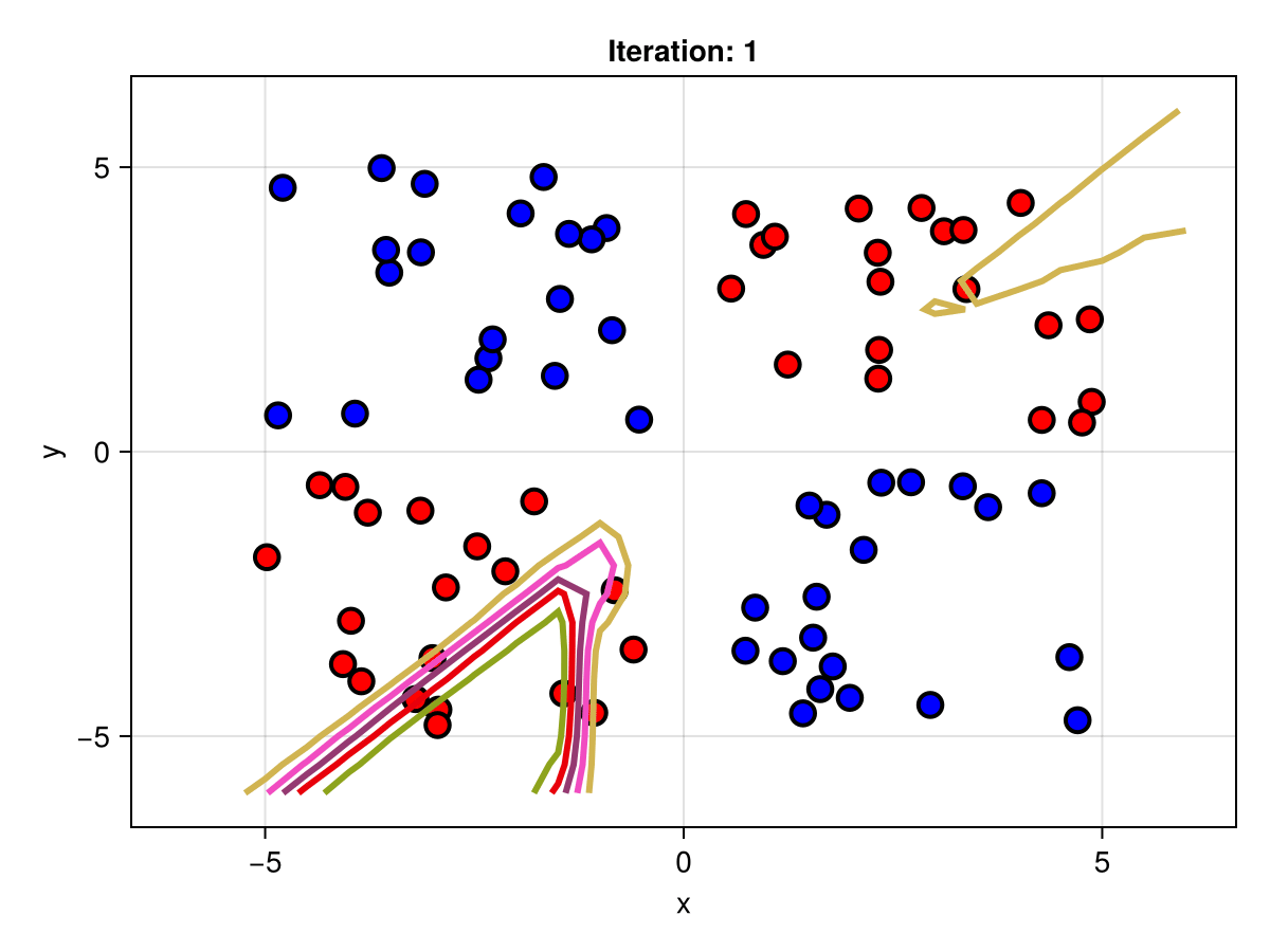

Appendix

using InteractiveUtils
InteractiveUtils.versioninfo()

if @isdefined(LuxDeviceUtils)
    if @isdefined(CUDA) && LuxDeviceUtils.functional(LuxCUDADevice)
        println()
        CUDA.versioninfo()
    end

    if @isdefined(AMDGPU) && LuxDeviceUtils.functional(LuxAMDGPUDevice)
        println()
        AMDGPU.versioninfo()
    end
end

Julia Version 1.10.5
Commit 6f3fdf7b362 (2024-08-27 14:19 UTC)
Build Info:
  Official https://julialang.org/ release
Platform Info:
  OS: Linux (x86_64-linux-gnu)
  CPU: 48 × AMD EPYC 7402 24-Core Processor
  WORD_SIZE: 64
  LIBM: libopenlibm
  LLVM: libLLVM-15.0.7 (ORCJIT, znver2)
Threads: 4 default, 0 interactive, 2 GC (on 2 virtual cores)
Environment:
  JULIA_CPU_THREADS = 2
  JULIA_DEPOT_PATH = /root/.cache/julia-buildkite-plugin/depots/01872db4-8c79-43af-ab7d-12abac4f24f6
  LD_LIBRARY_PATH = /usr/local/nvidia/lib:/usr/local/nvidia/lib64
  JULIA_PKG_SERVER = 
  JULIA_NUM_THREADS = 4
  JULIA_CUDA_HARD_MEMORY_LIMIT = 100%
  JULIA_PKG_PRECOMPILE_AUTO = 0
  JULIA_DEBUG = Literate

---

This page was generated using Literate.jl.