Visualizing Lux Models using Model Explorer

We can use model explorer to visualize both Lux models and the corresponding gradient expressions. To do this we just need to compile our model using Reactant and save the resulting mlir file.

using Lux, Reactant, Enzyme, Random

dev = reactant_device(; force=true)

model = Chain(
    Chain(
        Conv((3, 3), 3 => 32, relu; pad=SamePad()),
        BatchNorm(32),
    ),
    FlattenLayer(),
    Dense(32 * 32 * 32 => 32, tanh),
    BatchNorm(32),
    Dense(32 => 10)
)
ps, st = Lux.setup(Random.default_rng(), model) |> dev

x = randn(Float32, 32, 32, 3, 4) |> dev

Following instructions from exporting lux models to stablehlo we can save the mlir file.

hlo = @code_hlo model(x, ps, Lux.testmode(st))

write("exported_lux_model.mlir", string(hlo))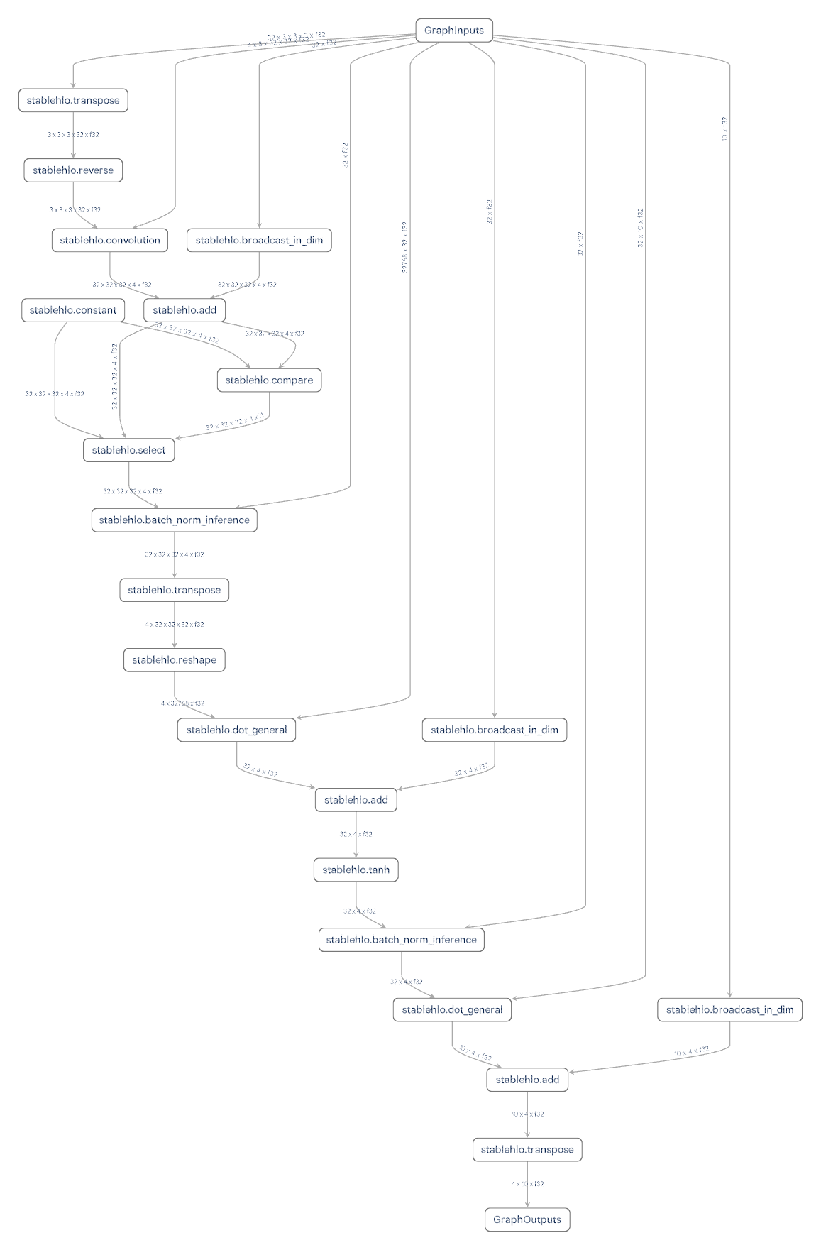

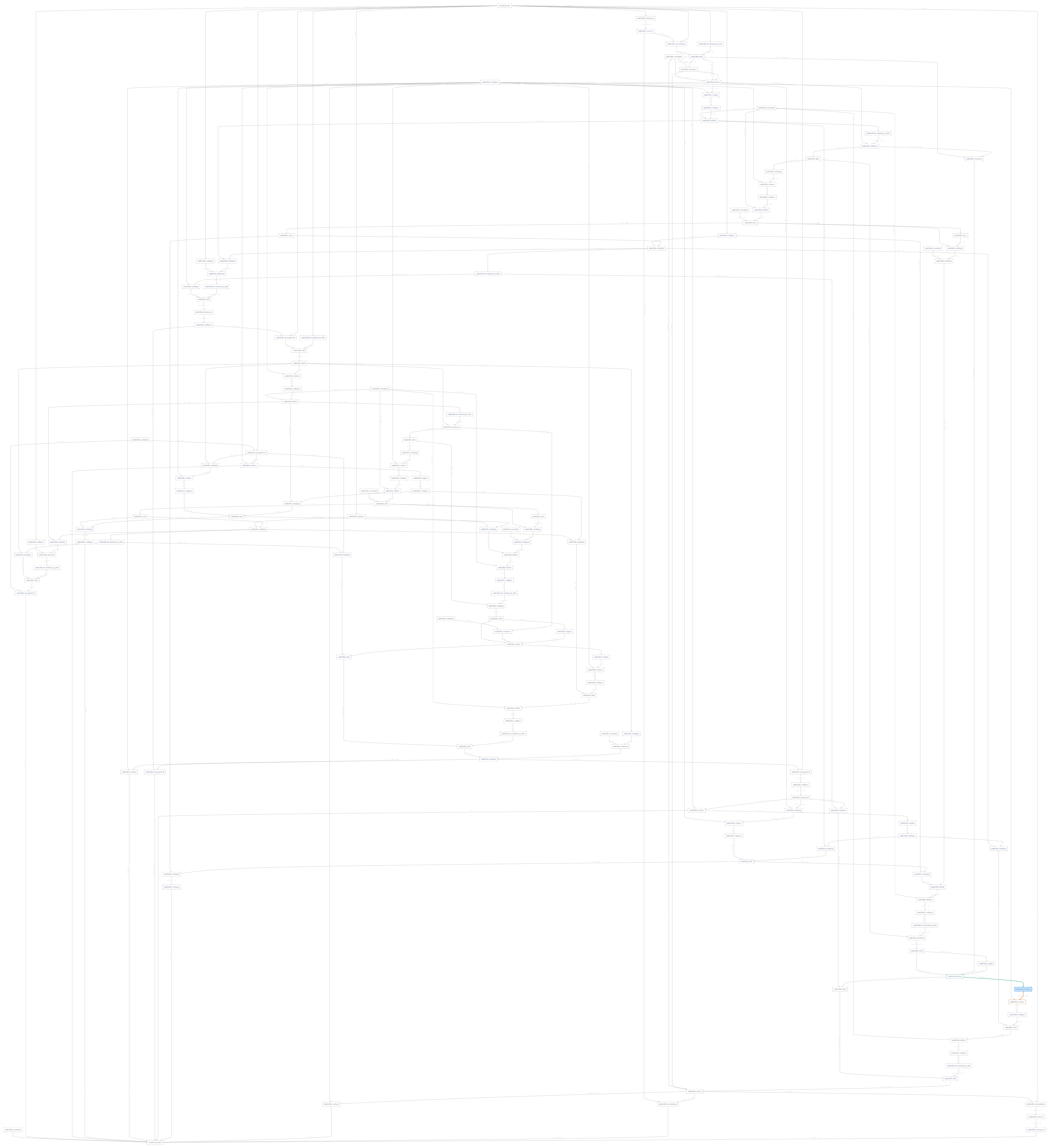
We can also visualize the gradients of the model using the same method.

function ∇sumabs2_enzyme(model, x, ps, st)
    return Enzyme.gradient(Enzyme.Reverse, sum ∘ first ∘ Lux.apply, Const(model),
        x, ps, Const(st))
end

hlo = @code_hlo ∇sumabs2_enzyme(model, x, ps, st)

write("exported_lux_model_gradients.mlir", string(hlo))

┌ Warning: `training` is set to `Val{true}()` but is not being used within an autodiff call (gradient, jacobian, etc...). This will be slow. If you are using a `Lux.jl` model, set it to inference (test) mode using `LuxCore.testmode`. Reliance on this behavior is discouraged, and is not guaranteed by Semantic Versioning, and might be removed without a deprecation cycle. It is recommended to fix this issue in your code.
└ @ LuxLib.Utils /var/lib/buildkite-agent/builds/gpuci-5/julialang/lux-dot-jl/lib/LuxLib/src/utils.jl:334

This is going to be hard to read, but you get the idea.